16376194
| Question | Answer |
| Chapter 1 Data Collection | Summary Points |
| Population | whole set of items that are of interest |
| Census | observes or measures every member of the population |
| Sample | selection of observations taken from a subset of the population used to find info about the population as a whole |
| Sampling Units | individual units of a population |
| Sampling frame | the list of sampling units in named or numbered form |
| simple random sample | one where every sample of size n has an even chance of being selected |
| systematic sampling | required elements are taken at regular intervals from an ordered list, eg. every 5th person |
| stratified sampling | population is divided into mutually exclusive strata, eg. male and female, and a random sample is taken from each |
| quota sampling | an interviewer selects a sample that reflects the characteristics of the whole population |
| opportunity sampling | taking the sample from people who are available at the time the study is carried out and who fit the criteria you are looking for |
| quantitative data/variables | numerical observations |
| qualitative data/variables | non-numerical observations, ie. words |
| continuous variable | a variable that can take any value in a given range, ie. height |
| discreet variable | a variable that can take only specific values in a given range, ie shoe size |
| classes | in grouped frequency tables, specific values are not shown, groups are called classes |
| class boundaries | maximum and minimum values that belong in that class |
| midpoint | average of the class boundaries |
| class width | difference between upper and lower class boundaries |
| Chapter 2 Measures of location and spread | Summary points |
| mode/modal class | value that occurs the most |
| median | middle value when data ordered, take an average if there are two values |
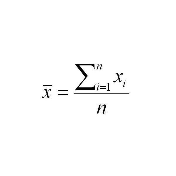
| mean | |
| for a mean in a frequency table | |
| lower quartile for discrete data | divide n by 4, if a whole number, Q1 is halfway between this data point and the next one up, if not round up and pick that point |
| upper quartile for discreet data | find 3/4 n, if a whole number, Q3 is halfway between this data point and the next one up, if not round up and pick that point |
| range | difference between min and max value |
| IQR | Q3 - Q1 |
| Interpercentile range | difference between the values for two given percentages |
| Variance | see textbook p39 |
| Standard Deviation | square root of variance |
| Variance and Standard Deviation in a frequency table | See textbook p39 |
| mean of coded data | see textbook p39, (do as coded formula says) |
| standard deviation of coded data | see textbook p39, (only multiply divide, don't add or subtract) |
| Chapter 3 Representations of data | Summary Points |
| outlier | greater than Q3 + k (IQR) less than Q1 - k (IQR) |
| cleaning data | this is the process of removing anomalies from data |
| frequency density (height of bar) | on a histogram, area of bar = k x frequency |
| frequency polygon | formed by joining the middle of the top of each bar in a histogram with equal class widths |
| comparing data sets | comment on: 1 measure of spread 1 measure of location |
| Chapter 4 Correlation | Summary Points |
| bivariate data | data has pairs of values for two variables |
| Correlation | describes linear relationship between two variables |
| Regression line | written in the form y = a + bx |
| the coefficient b | tell you the change in y for each unit change in x, if positive correlation b is positive and vice versa |
| Interpolation and Extrapolation | only use the regression line for interpolation, not extrapolation |
| Chapter 5 Probability | Summary Points |
| Venn diagram | represents events graphically, frequencies or probabilities can be placed in a venn diagram |
| mutually exclusive events | P(A or B) = P(A) + P(B) |
| independent events | P(A and B) = P(A) x P(B) |
| tree diagram | used to show the outcomes of two (or more) events happening in succession |
| Chapter 6 Statistical Distribution | Summary Points |
| Probability distribution | fully describes probability of any outcome in the sample space |
| sum of probabilities | sum of probabilities must always add up to 1 |
| Binomial distribution, B(n,p) | X can be modelled with a Binomial Distribution if: there are a fixed number of trials, n there are only two possible outcomes there is a fixed probability of success the trials are independent of each other |
| probability mass function | see page 97 for formula |
| Chapter 7 Hypothesis Testing | Summary Points |
| Ho, null hypothesis | assume this hypothesis to be correct eg. Ho: p=0.7 |
| H1, alternate hypothesis | tells us about the parameter if assumption is shown to be wrong, eg. H1: p>0.7 |
| One tailed | where p< or p> |
| Two tailed | p is not equal to |
| critical region | if the test statistic falls within this region reject H0 accept H1 |
| critical value | first value to fall inside of the critical region remember for upper boundary it is 1 - P(x less than or equal to y), can be found using tables or calculator |
| actual significance level | probability of an event happening by chance |
| two-tailed test | critical region is split at either end of distribution, half significance level at end you are testing |
Want to create your own Flashcards for free with GoConqr? Learn more.